Introduction to Flow Matching

Why learn about flow matching?

Flow matching [5] is truly a gem inside the modern theory of generative modeling. It is a simple, elegant and remarkably powerful algorithm that allows us to efficiently sample from highly complex distributions. These can be any distributions we like! Images, video, voice data, you name it. This is why these methods have found applications in so many domains and currently dominate the state-of-the-art.

The field did not suddenly stumble upon flow matching. The theory and understanding of generative modeling has evolved throughout the last 3 decades through a wide variety of perspectives. In fact, it is still evolving: flow matching is one way of doing things, and not necessarily the best way. Nonetheless, it is a vital tool that should exist in the arsenal of the modern computer scientist.

Plus, it’s quite easy to grasp and even easier to implement! So, without further ado, let’s learn all about it!

Outline

The tutorial in this page is long. I’ve tried to organize it in a bottom-up fashion, but it still relatively dense. One way to work through it is via 3 stages: (1) understanding the intuition behind flow matching, (2) going through the rigorous mathematical details, (3) learning about different model architectures. Good luck 🙂

The Game Plan

Flow matching is an algorithm used in generative probabilistic modeling. The goal is to generate samples $z \sim p_{data}$ from an unknown distribution. Imagine this as generating pictures of dogs or sentences similar to Shakespearean works. There are numerous ways to achieve this, but we will examine the following viewpoint:

Flows, ODEs and Vector Fields

How do we learn a set of trajectories that transform one distribution to another?

In modern deep learning whenever we are asked about how to learn something, we usually think in two steps:

1. How do we represent the information
2. How can a neural network express and learn that representation.

We will first tackle the first step: representation

Trajectories arise naturally as solutions to ordinary differential equations (ODEs). These equations specify precisely two things we need to fully define trajectories:

• The initial point of the trajectory.
• For each point $(x,t)$ in space-time, the gradient of the trajectory at that point.

Let $u:\mathbb{R}^d\times [0,1] \to \mathbb{R}^d$ with $(x,t) \mapsto u_t(x)$ be a vector field specifying these constraints. It tells us for each point in time and space, not where the point is, but what its “velocity” is. This is captured by this ODE:

$$ \frac{d}{dt}X_t = u_t(X_t), X_0=x_0, $$

whose solution is a trajectory. Note that the “velocity” vector field depends both on time and space! The velocity at a given point in space changes as time passes!

• [Mathematical Interlude] Existence and Uniqueness of solutions to ODEs

  “Well-behaved” ODEs are guaranteed to have unique solutions within a local domain. We typically constrain $t \in [0,1]$ and assume that $u$ is continuously differentiable with bounded derivative. In those cases the Picard-Lindelöf theorem guarantees that the ODE written above has a unique solution.

If we let the starting point be a parameter then we can ask where the point is at time $t$ if it started at $x_0$. This is given by a function called the flow :

$$ \psi:\mathbb{R}^d\times [0,1]\to\mathbb{R}^d, (x_0,t)\mapsto \psi_t(x_0)\\ \frac{d}{d}\psi_t(x_0)=u_t(\psi_t(x_0)), \psi_0(x_0)=x_0 $$

A flow defines multiple trajectories, one per initial point and a corresponding ODE. For soundness’ sake, it is true that when $u$ is a continuously differentiable vector field with bounded derivatives, then the ODE has a unique solution given by the flow.

Solving ODEs numerically is a well-studied topic. One of the simplest ways to do is simulate the ODE through finite differences via Euler’s method. This relies on the definition of the derivative as the limit of average speed over an infinitesimal time period:

$$ X_{t+h} = X_t + hu_t(X_t) $$

There are other methods to numerically solve ODEs, though we will not need to survey them here.

Flow Matching: An Intuitive Dive

Let’s try to build intuition first. We’ll ignore mathematical details and derivations for this section and try to develop an understanding of what these models try to do and how they are trained. Really, at the root of it, once one decides to accept this big assumption that we talked about earlier, they are, in a way, almost forced to do things in the way we outline below. It figures: this is what the field has converged to after almost 3 decades of research.

Returning, then, to our big assumption:

Conditional Velocity Fields

The big question is: How can we learn $u_t^\theta$?

Let’s try to imagine what happens during training: we have a dataset full of points sampled from $p_{data}$. In order to witness trajectories from $p_{init}$ we must somehow observe “intermediate” points $z_t$ on those trajectories. For example, if $x_1 \sim p_{data}$ is an image of a dog, imagine $z_t$ at $t \in (0,1)$ as a partially blurry version of $x_1$. At $t=0$ that image will be full noise, corresponding to distribution $p_{init}$.

We will cover the specifics of how $z_t$ is observed later on. Once a collection of intermediate points $z_t$ has been observed we need a way to tell our neural network: “at this point in space-time, this is the value of the velocity field”. Then we can define a regression-based loss function and let gradient descent do the rest.

So really the problem is: how do we read off the value of the velocity field at a given point in space time?

The most “obvious” answer is: recover the vector pointing back towards $x_1$.

Remember this as the “obvious” loss: try to get the neural network to predict the path back to a specific $x_1$.

Let’s call this the conditional velocity field $u_t(z_t \mid x_1)$. This is something we can easily compute since we are the ones who transformed $x_1$ into $z_t$.

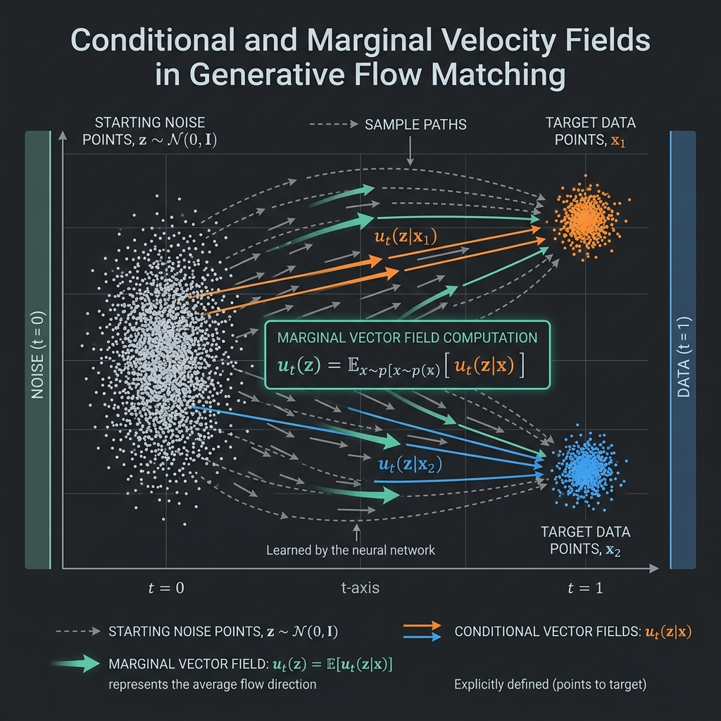
However! That is not the velocity field we want! It’s just the velocity field that takes trajectories to $x_1$! If we started from a different point, say $x_2$, and somehow recovered the same intermediate trajectory point $z_t$, the conditional velocity field $u_t(z_t \mid x_2)$ would be different as it would point towards $x_2$ instead. So, which field should our network prefer to learn?

It might be clear to you at this point, but the answer is: neither! We don’t want a velocity field taking us to any specific point, but rather a velocity field taking us to the $p_{data}$ distribution. One field to rule them all 🙂

Think of each conditional velocity vector as a specific “outcome”: if we follow it we end up at some data point $x_1$. The distribution over data points that we seek is $p_{data}$. Therefore, we should in general move towards the average direction over all outcomes, where each conditional velocity is weighted by the probability $q(x_1 \mid z_t)$ we end up at a specific outcome (we’ll talk about those weights in a second).

$$ u_t(z_t) = \mathbb{E}_{x_1 \sim q(x_1\mid z_t)}[u_t(z_t\mid x_1)] $$

This equation is simply the law of total probability re-written: we can recover the marginal distribution from the conditional distributions.

The Marginalization Trick

So our neural network will try to approximate $u_t(z_t)$. Given a point $z_t$ and time $t$ the neural network can regress on the value $u_t(z_t)$:

$$ \mathcal{L} = \mathbb{E}_{t,z_t}[||u_t^\theta(z_t)-u_t(z_t)||_2^2] $$

where we sample $t$ uniformly in $(0,1)$ and $z_t$ be an intermediate point sampled by repeatedly sampling $x_1 \sim p_{data}$ and blurring it. We will call this the Flow Matching (FM) loss.

The issue is that computing $u_t(z_t)$ is not tractable? Why? Because we don’t know the weights in the averaging calculation. Come to think of it, what distribution even is this $q(x_1 \mid z_t)$? The only distributions we have defined so far are $p_{init}$ and $p_{data}$. We’ll give a more rigorous treatment later in the article, but for now let’s stick to intuition:

How do we calculate for each $x_1$ the probability of it being obtained as a continuation of a trajectory starting at $z_t$ at time $t$?

We could use Bayes’ rule:

$$ q(x_1 \mid z_t) = \frac{q(z_t \mid x_1) \cdot q(x_1)}{q(z_t)} $$

• $q(z_t \mid x_1)$ is just easy to calculate as it corresponds to the “blurring” of an image, which we can control.
• $q(x_1)\equiv p_{data}$ is technically “easy” to get also: Draw a large sample of $N$ data points and use Monte-Carlo approximation. This can be done once and re-used.
• $q(z_t)$ → This is the painful one. What is the marginal probability of passing through $z_t$ at time $t$? We’d need to go over every single point in our dataset, “blur” it and integrate. This must be done every single time we need to calculate $u_t(z_t)$! Training would just be too slow.

Even though it is called the marginalization trick, there is really no trick to overcoming this situation. We are saved purely due to the will of the gods of probability.

Instead of computing $\mathcal{L}$ we will do what we simply, and without any additional fuss, go back and compute the obvious loss instead!

But wait! All this discussion was to tell you that the “obvious” loss doesn’t work. The thing is, you don’t have the network approximate the direction back to a single, fixed $x_1$. That would fail. We will instead approximate all the conditional velocity vectors simultaneously! We will call this the Conditional Flow Matching (CFM) loss.

$$ \mathcal{L}_{CFM} = \mathbb{E}_{t,z_t,x_1}[||u_t^\theta(z_t)-u_t(z_t\mid x_1)||_2^2] $$

where now we also sample $x_1$ as the “end goal” of the trajectory $z_t$ goes through.

We will soon prove that minimizing $\mathcal{L}_{CFM}$ is equivalent to minimizing $\mathcal{L}$! Isn’t that amazing! We turned an otherwise intractable problem to one that can be solved efficiently without sacrificing anything! That’s a rare occurrence in Machine Learning.

Moving Forward…

We have now a loss we can minimize via gradient descent, meaning we can train a model to represent the velocity field. Inference will be a piece of cake: just start from $p_{init}$ and apply the velocity field via the Euler method (for instance).

But there are still questions we have purposefully left unanswered in this first intuitive dive:

1. How do we “blur” data points into intermediates? How do we compute the target conditional velocities $u_t(z_t \mid x_1)$?
2. What are these “intermediate” distributions $q_t(x_1 \mid z_t)$?
3. What models will we use to best represent the velocity fields?
4. How many steps do we need to solve the ODE?

All we have so far is an intuitive understanding. Time to build the mathematical tools required to fully outline the algorithms involved in flow matching models.

Flow Matching: A Deep Dive

We will trace the intuitive analysis we gave above and formalize everything.

1) Conditional and Marginal Probability Paths

The formal way to think about how we transform $p_{init}$ to $p_{data}$ is through probability paths. At each timestep of such a path we have an intermediate probability distribution $p_t$, with $X_0 \sim p_{init}$ and $X_1 \sim p_{data}$.

When we fixed the “outcome” of the flow to be some point $z \in \mathbb{R}^d$ we essentially restricted the final distribution to a deterministic Dirac spike $\delta_z$. Then the conditional probability path is a collection of distributions $p_t(x \mid z)$ over $\mathbb{R}^d$ such that $p_0(\cdot \mid z) = p_{init}$ and $p_1(\cdot \mid z) = \delta_z$ for all $z$. We are in control of what these look like and we will choose them to be tractable and easy to work with (see Gaussian paths later on)

Conditional paths lead straight away to marginal ones by applying the law of total probability. All we have to do is sample $z \sim p_{data}$ and $x \sim p_t(\cdot \mid z)$. This gives us $x \sim p_t$. The density is given via a simple integration, though it is intractable to actually compute.

$$ p_t(x) = \int p_t(x\mid z)p_{data}(z)dz $$

These marginal paths are the ones we want: they interpolate between $p_{init}$ and $p_{data}$.

Let’s see the prototypical example:

Gaussian Conditional Paths

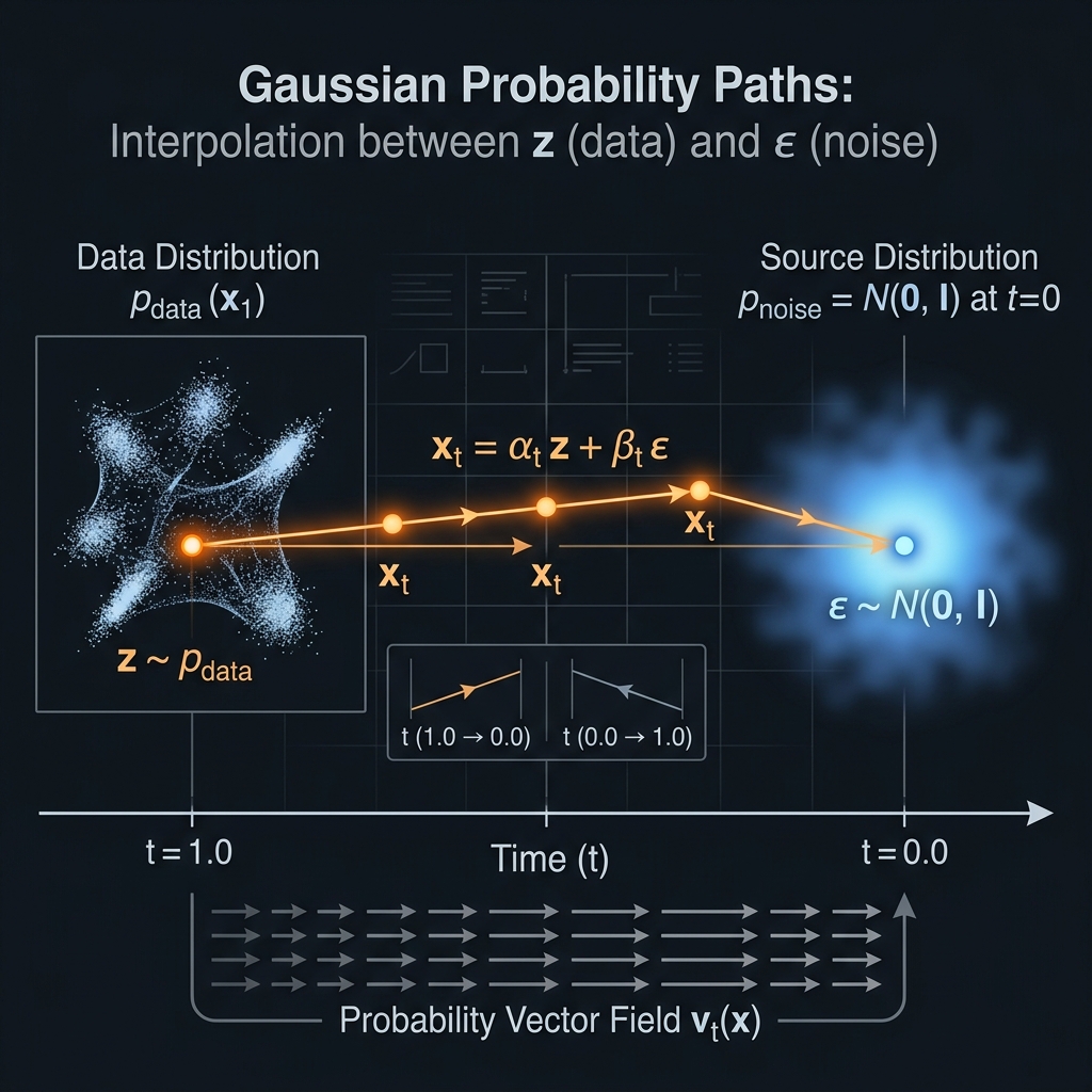
Let $\alpha_t$ and $\beta_t$ be noise schedulers: continuously differentiable, monotonic functions with $\alpha_0 = \beta_1 = 0$ and $\alpha_1 = \beta_0 = 1$. Then let

$$ p_t(\cdot \mid z) = \mathcal{N}(\alpha_t z, \beta_t^2 I_d) $$

Note that as the variance decreases to zero and the mean grows to one, this fulfills:

• $p_0(\cdot \mid z) = \mathcal{N}(0, I_d) = p_{init}$
• $p_1(\cdot \mid z) = \delta_z$

So it is a perfectly good conditional probability path!

Thus, how do we sample from the marginal path?

Easy! Just use the properties of the Gaussian distribution and the sampling process we described earlier: $z \sim p_{data}, \varepsilon \sim p_{init} = \mathcal{N}(0,I_d)\implies \boxed{x = \alpha_t z + \beta_t \varepsilon \sim p_t}$

This gives us one missing piece of the puzzle: how to apply noise and get the intermediate point $z_t$ (here written as $x$)

2) Conditional and Marginal Velocity Fields

Now on to the conditional velocity fields. These are as we imagined them earlier: fix an outcome $z$ and define a vector field $u_t(\cdot \mid z)$ whose corresponding ODE yields trajectories on the conditional probability path $p_t(\cdot \mid z)$

$$ X_0 \sim p_{init},\frac{d}{dt}X_t = u_t(X_t\mid z) \implies X_t \sim p_t(\cdot \mid z) $$

As we did before, we can marginalize these conditional vector fields to get marginal vector fields. All we need to do is sample $z$. Expanding using Bayes’ rule suggests that:

$$ u_t(x) = \int u_t(x\mid z)\frac{p_t(x\mid z)p_{data}(z)}{p_t(x)}dz. $$

This field follows the marginal probability path, i.e.

$$ X_0 \sim p_{init},\frac{d}{dt}X_t = u_t(X_t) \implies X_t \sim p_t $$

• Proof of the equivalence:

  We use the following mathematical tool that relies on the divergence operator. That operator is a scalar field, adding up the partial derivatives along all components of a vector field. We can think of it intuitively as representing fluid flow:

  $$ \text{div}(u_t)(x)=\sum\limits_{i=1}^d\frac{\partial}{\partial x_i} u_t^{(i)}(x) $$

  
  Continuity Equation
  
  
  $X_t \sim p_t$ for all $0 \leq t \leq 1$ if and only if
  
  
  $$ \partial_t p_t(x) = -\text{div}(p_t u_t)(x) $$
  for all $x \in \mathbb{R}^d$ and $t$.
  

  Think of this via a physical analogue: the rate of change in density of a fluid field is always the negative of the divergence of the mass flux vector: $\partial\rho/\partial t = -\nabla\cdot (\rho v)$. We can think of the probability through time as such a fluid and $u_t$ as its velocity field.

  We will defer the proof of the continuity equation to a subsequent writing. It is encompassed by the Fokker-Planck theorem for SDEs.

  So all we have to do is show that our marginal vector field satisfies the continuity equation. This is done by direct calculation:

  $$ \partial_t p_t(x) = \partial_t \int p_t(x\mid z)p_{data}(z)dz = \int \partial_t p_t(x\mid z)p_{data}(z)dz\\ = \int-\text{div}(p_t(\cdot \mid z)u_t(\cdot \mid z))(x) p_{data}(z)dz $$

  because we can apply the continuity equation to $p_t(x \mid z)$ as well. Then we have:

  $$ =-\text{div}\left(\int p_t(x\mid z)u_t(x \mid z) p_{data}(z)dz \right)\\ = -\text{div}\left(p_t(x)\int u_t(x\mid z)\frac{p_t(x\mid z)p_{data}(z)}{p_t(x)}dz\right)\\ = -\text{div}(p_t u_t)(x) $$

  as required.

This is the field that converts $p_{init}$ to $p_{data}$.

This is what we want our neural network to learn.

This is, for all intents and purposes, our generative model.

Conditional Velocity Fields for Gaussian Paths

Since we’re running with the Gaussian probability paths, we should see how they translate to the conditional velocity fields. This is vital — it will give us the targets we were seeking for the CFM loss.

Recall that $p_t(\cdot \mid z) = \mathcal{N}(\alpha_t z, \beta_t^2 I_d)$. Let $\dot{\alpha}_t = \partial_t\alpha_t$ and $\dot{\beta}_t = \partial_t \beta_t$. We wish to figure out $u_t(x\mid z)$. Start by letting $\psi_t(x\mid z) = \alpha_t z + \beta_t x$ the the trajectory that links the sampled $X_0 \sim p_{init}$ to the conditioned $z$. Then let’s plug into the ODE:

$$ \frac{d}{dt}\psi_t(x\mid z) = u_t(\psi_t(x\mid z)\mid z)\iff\\ \dot{\alpha}_t z+\dot{\beta}_t x = u_t(\alpha_t z + \beta_t x\mid z) $$

Now we only need to reparameterize $x\to (x-\alpha_t z)/\beta_t$ to get

$$ \boxed{u_t(x\mid z) = \dot{\alpha}_t z+\dot{\beta}_t\left(\frac{x-\alpha_t z}{\beta_t}\right)} $$

3) Flow Matching Losses

As we discussed, the flow matching loss is defined as:

$$ \mathcal{L}_{FM} = \mathbb{E}_{t\sim\text{unif}, x\sim p_t}[||u_t^\theta(x)-u_t(x)||_2^2] $$

Note that sampling from $p_t$ is easy given the conditional probability paths: $z\sim p_{data}, x\sim p_t(\cdot \mid z)$. As we saw, this loss is intractable to compute, so we define the conditional flow matching loss:

$$ \mathcal{L}_{CFM}(\theta)=\mathbb{E}_{t,z,x}[||u_t^\theta(x)-u_t(x\mid z)||_2^2]. $$

Time to understand why minimizing the latter works for minimizing the former.

As a result, the gradients are the same and minimizing one via SGD is the same as minimizing the other.

Proof

We just need to stare at what is being calculated and do some re-shuffling:

$$ \mathcal{L}_{FM}(\theta)=\mathbb{E}_{t,x}[||u_t^\theta(x)||_2^2-2u_t^\theta(x)^\top u_t(x) + ||u_t(x)||_2^2]\\ =\mathbb{E}_{t,z,x}[||u_t^\theta(x)||^2]-2\mathbb{E}_{t,x}[u_t^\theta(x)^\top u_t(x)] + C_1 $$

where $\mathbb{E}[||u_t(x)||_2^2]$ is a constant $C_1$ with respect to $\theta$. Then we have:

$$ \mathbb{E}_{t,x}[u_t^\theta(x)^\top u_t(x)] =\int_{0}^1\int p_t(x)u_t^\theta(x)^\top u_t(x)dx dt\\ =\int_0^1\int p_t(x)u_t^\theta(x)^\top\left[\int u_t(x\mid z)\frac{p_t(x\mid z)p_{data}(z)}{p_t(x)} dz\right] dx dt\\ =\int_0^1\int \int u_t^\theta(x)^\top u_t(x\mid z)p_t(x\mid z)p_{data}(z)dzdx dt\\ =\mathbb{E}_{t,z,x}[u_t^\theta(x)^\top u_t(x\mid z)] $$

Then adding and subtracting $||u_t(x\mid z)||_2^2$ allows us to re-write:

$$ \mathcal{L}_{FM}(\theta) = \mathbb{E}_{t,z,x}[||u_t^\theta(x)-u_t(x\mid z)||_2^2] + \mathbb{E}_{t,z,x}[-||u_t(x\mid z)||_2^2]+C_1 $$

Since $\mathbb{E}_{t,z,x}[-||u_t(x\mid z)||_2^2]$ is another constant, our claim is proved.

4) Full Training and Inference Algorithms

We are now finally able to conclude our deep dive through flow matching models by providing precise algorithms for training and inference.

Recall that we have chosen to use Gaussian probability paths: $p_t(\cdot \mid z) = \mathcal{N}(\alpha_t z, \beta_t^2 I_d)$, so we can sample $x_t = \alpha_t z + \beta_t \varepsilon$ for $\varepsilon \sim \mathcal{N}(0,I_d)$. We derived the conditional vector field $u_t(x\mid z) = (\dot{\alpha}_t - \dot{\beta}_t\alpha_t/\beta_t)z + (\dot{\beta}_t/\beta_t)x$, meaning we can plug that into the CFM loss:

$$ \mathcal{L}_{CFM}(\theta) = \mathbb{E}_{t,z,x}[||u_t^\theta(x)-u_t(x\mid z)||_2^2]\\ =\mathbb{E}_{t,z,\varepsilon\sim\mathcal{N}(0,I_d)}[||u_t^\theta(\alpha_t z+\beta_t \varepsilon)-(\dot{\alpha}_t z+\dot{\beta}_t \varepsilon)||_2^2] $$

A simple case would be when $\alpha_t = t$ and $\beta_t = 1-t$. Then this reduces to:

$$ \mathcal{L}_{CFM}(\theta)=\mathbb{E}_{t,z,\varepsilon}[||u_t^\theta(tz+(1-t)\varepsilon)-(z-\varepsilon)||_2^2] $$

In other words, the “predicted” instantaneous velocity at the interpolated point on the line between $z$ and $\varepsilon$ tries to match the actual slope of the line $z-\varepsilon$.

Training

For each mini-batch of data:
1. Sample $t\sim \text{Unif}(0,1)$, $\varepsilon\sim\mathcal{N}(0,I_d)$ and $z$ from the dataset.
2. Compute the loss $\mathcal{L}(\theta) = ||u_t^\theta(tz + (1-t)\varepsilon) - (z-\varepsilon)||_2^2$
3. Apply a gradient update.

It’s really as simple as that! Inference is even simpler.

Inference

1. Set $t=0$ and let $h=1/n$ be a step size.
2. Draw a sample $X_0\sim \mathcal{N}(0,I_d)$.
3. for $i=1,…,n$ do:
   • $X_{t+h} = X_t + hu_t^\theta(X_t)$
   • $t \gets t+h$
4. return $X_1$

Where we stand

We have concluded an intuitive and technical deep dive into flow matching models. These are very powerful models under the “diffusion model” umbrella and are used commonly throughout many applications in language, computer vision, robotics and beyond. And now you understand fully how they work.

In retrospect, the main ideas are rather simple. It all boils down to this “big assumption” that we made in the beginning.

1. We assume that a smooth transformation exists between a convenient distribution such as the Gaussian and the distribution we want to sample from.
2. We imagine that transformation as a collection of trajectories taking points from Gaussian space to “image” space.
3. We represent these trajectories by using a velocity vector field and have a neural network try to express that field.
4. Learning a field that morphs distributions is hard (due to the intractability of the integrals involved). Instead, we focus on what we can observe: conditional trajectories. In most cases, these are just straight lines!
5. We use marginalization to show that regressing the neural network on conditional trajectories alone is equivalent to learning the velocity vector field that we aimed for in the beginning!

How do we actually make these models? Guidance and Neural Architectures

Now that we know the theory, let’s dive into practice. The main questions that we still haven’t answered are:

1. How do we steer the model towards a certain output? Our models so far are unguided — they generate some image. We want the ability to provide prompts.
2. What neural networks will work well and what architectures should we prefer for $u_t^\theta$?

Guidance

Suppose we have a prompt $y$ (for example a text prompt for generating images). We want to sample from $p_{data}(z\mid y)$. The vanilla way of doing this is to simply parameterize our neural network to accept prompts:

Neural Network: $(x,y,t) \mapsto u_t^\theta(x\mid y)$

Then we generate samples by following $u_t^\theta(X_t \mid y)$ for given prompt $y$.

For training, we can consider a guided CFM objective that allows us vision of all the conditional distributions:

$$ \mathcal{L}_{CFM}^{\text{guided}}(\theta) = \mathbb{E}_{(z,y)\sim p_{data}, t, x\sim p_t(\cdot \mid z)}||u_t^\theta(x \mid y) - u_t(x \mid z)||^2 $$

There is a problem here though: There are a lot of possible labels and our model is likely to underfit. Since prompt-based navigation throughout the latent space is difficult, we often end up with blurry images or strange artifacts. This is a price we pay for requiring the image generated to be faithful to the prompt.

We need a way to re-inforce the prompt variable $y$ while also preserving the generation quality of the unconditional vector field. The issue lies really in what we require the neural network to learn. If we want it to capture every conditional distribution $p_t(z\mid y)$ then we are asking too much. And thus the results we get are poor.

Enter classifier-free guidance, the state-of-the-art technique used here. The main idea is the following:

Instead of learning a guided velocity field, we interpret $u_t^\theta(x\mid y)$ as a steering direction that tells the unconditional velocity field how to navigate towards the part of the latent space that is mostly associated with the prompt.

Neural Network Architectures

The task now is to explore neural network architectures for modeling $u_t^\theta(x\mid y)$. The input is $(t,x,y)$ and the output is a vector in $\mathbb{R}^d$.

A) MLPs or CNNs

A simple way to start is just by using an MLP on the concatenation of $x,y$ and $t$. If the inputs are low-dimensional we could hope this actually is expressive enough to yield good results. We could use a convolutional neural network to kick things up a notch and help the network acquire spatial information for image or video data.

Alas, these networks are not expressive enough in most cases.

Modern pipelines rely heavily on attention. Enter the Diffusion Transformer (DiT) [4].

B) Diffusion Transformers (DiT)

Transformers are at this point a ubiquitous architecture. Really the main leap forward they provide is the ability to model “relationships” between different parts of the network. This makes the network a lot more expressive, allowing for complex latent spaces to emerge.

For the flow matching models we are studying, we need a way to leverage the attention mechanism to embed our input time-step $t$, prompt label $y$ and latent $x$.

1. Time Embedding: time is a single number between 0 and 1. Compare that to the huge vector spaces that the rest of our embeddings live in. Time could get easily “lost”. To force the network to pay attention to time, we embed it to a higher-dimensional subspace, typically by using Fourier Features:

   $$ \text{TimeEmbd}(t) = \sqrt{\frac{2}{d}}\left[\cos(2\pi w_1 t)\cdots \cos(2\pi w_{d/2}t)\sin(2\pi w_1 t)\cdots \sin (2\pi w_{d/2} t)\right] $$

   where $w_i = w_{\min} \left(\frac{w_{\max}}{w_{\min}}\right)^{(i-1)/(d/2 - 1)}$ are the frequencies. Note this embedding always has norm $1$, so you can think of it as a vector on the unit $d$-dimensional sphere.

   If you’re seeing it for the first time, this kind of embedding might seem mysterious. There are fundamental relationships to Random Fourier Features, RoPE embeddings and other areas of mathematics. I’ll devote another blog post to explaining them. But to get a sense of what’s happening, recall from simple trigonometry that the function $\cos(2\pi fx)$ is a sinusoidal wave with period $T=\frac{1}{f}$. The frequencies $w_i$ are geometrically distributed, so the first ones are really small, while the last ones are very large, with the gaps growing exponentially. Thus, the sinusoidal curves go from having really large period to really small period. This structure makes two things possible that we value:

   • Metric distances in the embedded space are relative, aka depend only on the distance in the time space, not the timesteps themselves.
   • With high and low frequencies both present, the network has a versatile sense of scale: it can tell the difference between large and small time scales.
     2. Embedding prompts: if the prompt is a class label $y \in [N]$, then we often learn a separate embedding vector for each class. If the prompt is text or more complicated, we often rely on more complicated models that embed the discrete prompt into a continuous space. A common feature-extraction model for text, for instance, is CLIP (Contrastive Language-Image Pre-training), which relies on a vision transformer to map both images and text into the same latent space.

   But really, this is a space where tricks emerge and imagination can take you far! Different modalities can benefit from different embeddings and structure. There is no one good recipe, and so we have a wide variety of models and approaches.
   

To embed the latent $x$, we will need to go through the DiT architecture itself. For this blog, we will work with images. The architecture is quite straightforward:

1. Split the image into $N$ patches of size $P\times P$.
2. Embed each patch into a $d$-dimensional token via a linear transformation.
3. Apply $L$ DiT Blocks to the patch, time and prompt embeddings using $H$-head attention.
4. De-patchify back to the desired output shape.

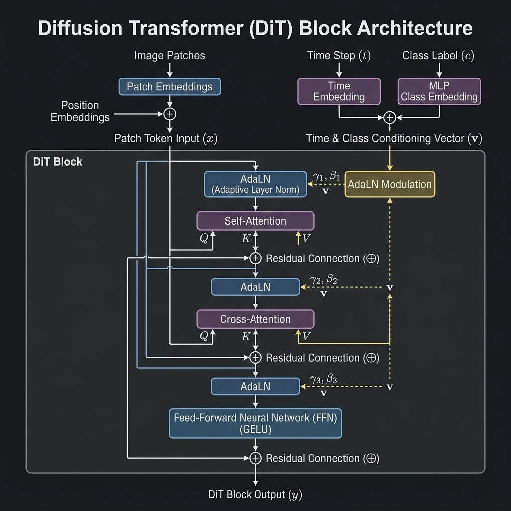
The heart is: how are DiT Blocks implemented? Here we rely largely on the attention mechanism. A typical DiT block contains the following ingredients:

1. Self-attention on patch tokens (of the latent $x$): queries, keys and values come from the latent $x$ tokens. The complexity here is $O(N^2)$.
2. Cross-attention to the prompt: here the latent $x$ are still the queries, but the keys and values are given by the token sequence in $y$. The complexity is $O(NM)$, where $M$ is the number of tokens in $y$.

3. Time Conditioning via Adaptive Normalization (AdaLN): Let $\tilde{t} \in \mathbb{R}^d$ be the timestep embedding. We typically use it to modulate normalized activations throughout the previous steps. First, we pass both the timestep and an aggregated $y$-conditioning vector $c$ through an MLP $g$ to get a vector in $2d$ dimensions:

   $$ (\gamma,\beta) = g(\tilde{t},c) $$

   Then, if $\text{Norm}$ is a normalization operator (like LayerNorm), we define:

   $$ \text{AdaNorm}_{\tilde{t}}(x) = (1+\gamma)\odot \text{Norm}(x)+\beta $$

   The key is that the scale $\gamma$ and shift $\beta$ is chosen dynamically based on the timestep. This is how the model decides which features are important depending on the time-scale.

   SOTA models use AdaLN-Zero, in which the MLPs also predict a scale parameter $\alpha$ for dimension-wise scaling. The linear layers in the MLP are crucially initialized to zero, making the block initially a pure identity function.

Putting it all together, here is an example DiT architecture based on what we’ve discussed so far:

• $x \gets x + g_1(\tilde{t},c) \odot \text{MHA}(\text{AdaNorm}_{\tilde{t}}(x),\text{AdaNorm}_{\tilde{t}}(x))$ → Self-Attention
• $x \gets x + g_2(\tilde{t},c)\odot \text{MHA}(\text{AdaNorm}_{\tilde{t}}(x), y)$ → Cross-Attn Conditioning
• $x \gets x + g_3(\tilde{t},c)\odot \text{MLP}(\text{AdaNorm}_{\tilde{t}}(x))$ → Residual connection

C) U-NETs

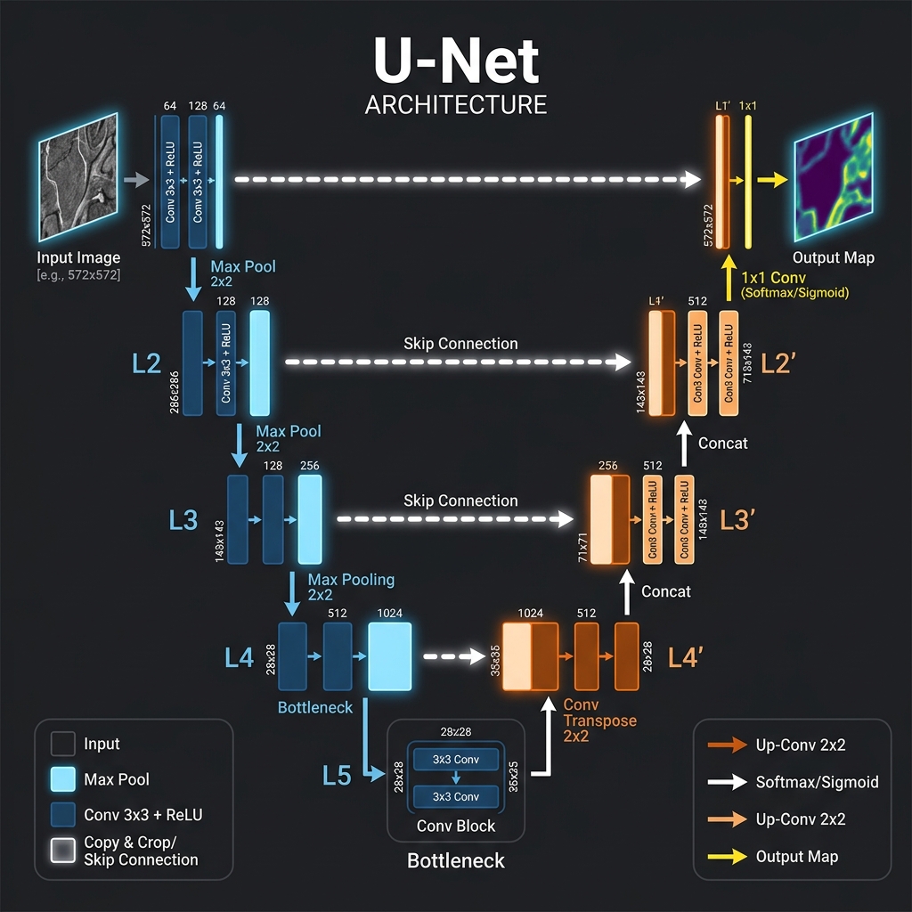
U-Nets are another architecture that is often seen. For really high-resolution images or bulky assets that are tokenized into a large number of tokens, they might be preferred over DiTs for speed. That being said, they are not as expressive and nowadays are not used as often.

U-Nets are convolutional neural networks. They take an image at high resolution (say $512 \times 512$) and “squeeze” it into a smaller space (say $32\times 32$), while also increasing the number of channels. Spatial information is converted directly to the embedding space. An encoder is used for downsampling, typically via max-pooling layers. A decoder uses up-convolutions to reconstruct the condensed information. A midcoder as well as residual connections between different parts, are often used.

I won’t get into more details, but understanding CNNs and U-Nets in general is important in computer-vision tasks, so I might make another quick blog about them.

D) Variational Autoencoders (VAEs)

The main issue with DiTs is that despite their power they need to “tokenize” the space. For example, this happens through “patches” in images. But when the resolution is really large, the number of tokens explodes and we can no longer afford the quadratic cost of attention. What is more, the sheer dimension of the velocity space explodes.

VAEs allow us to work directly in the latent space through compression. We teach a model to compress and reconstruct the data, while also retaining “regularity” in the latent space distribution. This is typically done via KL regularization. I wrote a whole other blog on VAEs here, if you are interested.

The VAE + DiT combo is very popular for generative modeling as of 2026. By reaching this point in the tutorial you are equipped to read most papers in the space! Things are changing, though — we are seeing lots more approaches generating directly in pixel space. After all, why train a VAE if we don’t need one?

Where to go next?

This constitutes a fairly comprehensive overview of flow matching models, how they work, why they work and how we can actually build them from zero. I promised blogs on a few topics throughout:

1. The mathematics of Fourier Features
2. CLIP embeddings and ViTs
3. CNNs and U-Nets

While I work on those, you can explore the fascinating world of generative modeling. With the tools we developed in this tutorial, you can explore the cutting-edge research pushing generative modeling to the limits.

Modern research directions with generation include:

• Reducing the number of (Euler) steps needed during inference. Here you’ll see approaches like consistency models [3,6] or meanflow [2] dominating the scene.
• Sculpting the latent space more efficiently. When generating points in highly specialized manifolds, we can modify the generation algorithms.
• Challenging the very core of our big-assumption: what is really the best way to parameterize the transformation between two distributions?

I also highly encourage you to check out the original papers outlining all these ideas! I included some of them below.

Till next time!

References

[1] Introduction to Flow Matching and Diffusion Models, Peter Holderrieth and Ezra Erives (2026), https://diffusion.csail.mit.edu/, 2506.02070 (arxiv)

[2] Geng, Zhengyang, et al. "Mean flows for one-step generative modeling." Advances in Neural Information Processing Systems 38 (2026): 75460-75482.

[3] Frans, Kevin, et al. "One step diffusion via shortcut models." International Conference on Learning Representations. Vol. 2025. 2025.

[4] Peebles, William, and Saining Xie. "Scalable diffusion models with transformers." Proceedings of the IEEE/CVF international conference on computer vision. 2023.

[5] Lipman, Yaron, Ricky TQ Chen, Heli Ben-Hamu, Maximilian Nickel, and Matt Le. "Flow matching for generative modeling." arXiv preprint arXiv:2210.02747 (2022).

[6] Cheng Lu and Yang Song. Simplifying, stabilizing and scaling continuous-time consistency models. In International Conference on Learning Representations (ICLR), 2025.