Reinforcement Learning: Foundations, Policy Gradients, and REINFORCE
June 2026
~20 min read
Themis Haris
Introduction
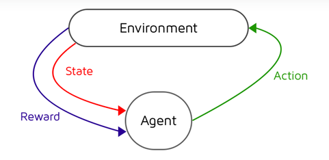
Reinforcement Learning (RL) is about developing algorithms to make decisions based on a
reward landscape. These algorithms yield so called policies, which are ways
to navigate complex state-space systems. The machine making decisions on behalf of a policy
is called an agent.
For example, consider the problem of teaching a machine to play Tetris. At each point in
time, the machine is faced with a state — what blocks have been laid out and what block is
on the way. It is also able to make a decision: where and how to place the incoming block.
Based on its decisions the state gets updated and the game continues.
Reinforcement learning is about teaching the agent how to play via a training
cycle of interactions with their environment.
This tutorial is a walkthrough over the fundamental algorithms and ideas that one needs to
know in order to get a solid foundation of RL. We will cover algorithms that show up
specifically in the context of deep learning, where we use neural networks to represent and
learn courses of action in complex systems.
Beyond the theoretical foundations, we will also look at implementation and see these
methods in practice. We will be using the Gymnasium library from OpenAI to
train an RL agent to do all sorts of cool things.
States, Actions and Markov Decision Processes
We will work in the following idealized setting. We consider a state space
$\mathcal{S}$, observation space $\mathcal{O}$ and
action space $\mathcal{A}$. These are sets that can be continuous (e.g. the
position of a robot) or discrete (e.g. a chess board). The observation space represents the
fact that we might not always be able to fully know the state we are in; instead we are only
equipped with the observations we make about the world.
Once inside these spaces, we imagine a time variable $t$ indexing the timestep we are in.
At time $t$, we are at state $s_t$ witnessing observation $o_t$. If we choose to take an
action $a_t \in \mathcal{A}$, then that action lands us in state $s_{t+1} \in \mathcal{S}$.
This gives a trajectory
$\tau = (s_1, a_1, s_2, a_2, \ldots, s_T)$ over a time-horizon with $T$ timesteps.
Once at state $s_t$, taking action $a_t$ doesn't deterministically take us to state
$s_{t+1}$. Instead we imagine that the next state is a random variable.
The probability of seeing state $s_{t+1}$ given we take action $a_t$ at state $s_t$ is
denoted by $p(s_{t+1} \mid s_t, a_t)$. These are called
transition probabilities.
A Markov Decision Process: states, actions, and probabilistic transitions.
Notice the enormous assumption we are making here: the next state depends only on
the previous state and the action we take! This is often called the
Markovian property. Indeed, we assume that the systems we are navigating
are so-called Markov Decision Processes (MDPs).
This is a huge assumption and is often not true in the real world. MDPs are
memoryless, since they forget about the past transcript and only care about the
most recent state and action. Our decisions in the real world very often carry memory. The
only way to incorporate memory in an MDP is by increasing the state space to include it,
which often makes the problem intractable.
Nevertheless, MDPs are a fundamental abstraction and we use them because of their
mathematical elegance. Many of the RL algorithms we will develop work well even if the
Markovian property does not hold.
Once the agent takes an action, it interacts with its environment and gets back a
reward $r(s_t, a_t)$. The goal of the agent is to learn a
policy $\pi(a_t \mid s_t)$ that will tell it which action to take at each
state. $\pi$ could be a probability distribution over actions and it could also depend on a
past window of observations: $\pi(a_t \mid o_{t-m:t})$.
Our goal will be to learn a policy that yields maximum reward over a
trajectory with horizon $T$. Note that the overall reward is what matters, not maximizing
the reward over a handful of actions. A central theme throughout will be the tradeoff
between exploration and exploitation: how do we
prioritize learning about the state space before making drastic decisions that will
"lock-in" our trajectory?
Imitation Learning
The first method we will cover is the simplest one: given a training set of example
trajectories from an expert, learn to imitate that expert. Despite its simplicity,
imitation is still a vital ingredient to training capable agents.
Key idea: We learn a policy $\pi(a \mid s)$ by parameterizing a neural
network to represent it. Then we just need to find the optimal parameters:
Recall that neural network architectures are really good at parameterizing distributions,
which is all $\pi(\cdot \mid s)$ is. We can use any kind of architecture we want here:
autoregressive models, diffusion, mixture of Gaussians, etc.
How do we solve this minimization problem? By collecting lots and lots of expert trajectories
and performing gradient descent. Since all the data is collected in advance, this type of
learning algorithm is called offline. Another name for this type of
imitation learning is behavior cloning.
The issue is that imitation learning requires
huge amounts of training data to capture every trajectory. Without enough
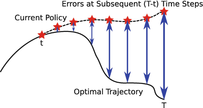
data we get compounding errors, where we find ourselves slowly escaping the
distribution we learned, with no way to get back.
Distribution shift: small errors compound over a trajectory, drifting far from the training distribution.
What if we learned how to correct the model if it leaves the right trajectory?
Methods that try to do this introduce interventions. They require an
extra step where we collect corrective data and then retrain.
DAgger (Dataset Aggregation) is a popular paradigm here.
Beyond the various difficulties with imitation learning, it faces another fundamental
obstacle: it cannot out-perform the demonstrator or allow for self-improvement. We will
need to do better.
Policy Gradients
We now present what is probably the most classic RL algorithm. The idea is quite
simple: why don't we treat this as any machine learning problem? Let's define a loss
function in terms of the reward and minimize it via gradient descent.
Recall that our goal was to maximize the expected reward over the long horizon.
Our final algorithm is simply gradient descent on this objective. The catch is:
every time we update $\theta$, our policy changes! So our trajectories need to be
re-collected! These algorithms are called on-policy because they
always act based on the data that the most recent policy has.
How do we re-use samples from previous policies? On a previous policy, the
probability of a trajectory is $\hat{p}(\tau)$. We have all this data — why not use it?
To use it, we employ a mathematical trick: $\mathbb{E}_{x \sim p}[f(x)] = \mathbb{E}_{x\sim q}\!\left[f(x)\cdot \frac{p(x)}{q(x)}\right]$
This way we can take a lot more gradient steps using the same data!
This isn't a silver bullet though — if we take too many gradient steps and our policy
changes significantly, our data no longer reflects trajectories that the new policies will
actually take. We need careful balancing here during training.
Implementation through Gymnasium
Time to see REINFORCE in action! We will write some code to use REINFORCE to learn a policy
for a lunar landing task. This task, as well as many others, are environments we can load
and easily interact with in Python through OpenAI's
Gymnasium library.
The Gymnasium Library
Gymnasium is fairly easy to use. You first instantiate an environment of your choice and seed it.
def make_env(env_id, seed=None, render_mode=None):
    env = gym.make(env_id, render_mode=render_mode)
    if seed is not None:
        env.reset(seed=seed)
        env.action_space.seed(seed)
        env.observation_space.seed(seed)
    return env
For our lunar lander, the state space and observation space are
identical. The state is [position, velocity, angle, angular velocity,
leg-contact booleans]. In general, the observation space might be missing
information and all we could do is treat it like the full state space.
Interactions are typically through a series of episodes:
obs, info = env.reset() — start a new episode, get the first observation.
obs, reward, terminated, truncated, info = env.step(action) — apply one action, get one timestep, collect the reward.
For the Lunar Lander, the reward is a built-in
variable: positive for moving toward the landing pad and reducing speed, points for
each leg touching down, a small fuel penalty per engine fire, and a large terminal
bonus/penalty (≈ +100 for a safe landing, ≈ −100 for a crash).
The full interaction loop looks like this:
obs, _ = env.reset()
ep_obs, ep_act, ep_rew = [], [], []
done = False
while not done:
    obs_t = torch.as_tensor(obs, dtype=torch.float32, device=device)

    # Sample an action from the current policy
    with torch.no_grad():
        dist = actor.distribution(obs_t)
        a = dist.sample()
    action = a.cpu().numpy()
    env_action = int(action) if is_discrete else action

    # Step the environment
    next_obs, reward, terminated, truncated, _ = env.step(env_action)
    ep_obs.append(obs)
    ep_act.append(action)
    ep_rew.append(reward)
    obs = next_obs
    done = terminated or truncated
This interaction is agnostic to the specifics of the task: we could be playing Atari
games, Tetris, or driving a car. The algorithms we write only see an interface of
actions and rewards.
Continuous vs. Discrete Spaces
If the action space is discrete, our actor outputs logits that we softmax over
(a Categorical distribution). If it is continuous, we output a mean and
variance and sample from a Gaussian.
class CategoricalActor(nn.Module):
    """Discrete policy: state -> logits -> Categorical distribution."""
    def __init__(self, obs_dim, n_actions, hidden=(64, 64)):
        super().__init__()
        self.logits_net = mlp([obs_dim, *hidden, n_actions], nn.Tanh)

    def distribution(self, obs):
        return Categorical(logits=self.logits_net(obs))


class GaussianActor(nn.Module):
    """Continuous policy: state -> Normal(mean, std).
    A single learnable log-std vector (not conditioned on the state)
    is the standard, stable choice for on-policy methods like PPO/A2C.
    """
    def __init__(self, obs_dim, act_dim, hidden=(64, 64)):
        super().__init__()
        self.mu_net  = mlp([obs_dim, *hidden, act_dim], nn.Tanh)
        self.log_std = nn.Parameter(-0.5 * torch.ones(act_dim))

    def distribution(self, obs):
        mu  = self.mu_net(obs)
        std = torch.exp(self.log_std)
        return Normal(mu, std)
The Lunar Landing task comes in two flavors in Gymnasium. We'll work with the
discrete one, where the possible actions are:
[do_nothing, left_engine, right_engine, main_engine].
We will be implementing on-policy REINFORCE. Recall the main training loop:
Collect data using the most recent policy (a batch of complete episodes).
Apply gradient updates using the surrogate objective:
$$\tilde{J}(\theta)\approx\frac{1}{N}\sum_{i=1}^N\sum_{t=1}^T\nabla_\theta\log \pi_\theta(a_{i,t}\mid s_{i,t})\left(\sum_{t'=t}^T r(s_{i,t'},a_{i,t'})-b\right)$$
First, some utility code to compute discounted prefix rewards up to time $t$.
We introduce a discount factor $\gamma$ here — you can treat it as $1$ for now.
def discount_cumsum(x, discount):
    """Compute discounted cumulative sums of a 1D array (right to left)."""
    out = np.zeros_like(x, dtype=np.float32)
    running = 0.0
    for t in reversed(range(len(x))):
        running = x[t] + discount * running
        out[t]  = running
    return out
Then the full training loop:
def policy_logp(obs_t, act_t):
    """Log prob of act_t under the current policy given obs_t."""
    dist = actor.distribution(obs_t)
    logp = dist.log_prob(act_t)
    if not is_discrete:
        logp = logp.sum(axis=-1)
    return logp


# ── Training ──────────────────────────────────────────────────
actor  = CategoricalActor(obs_dim, act_dim, hidden).to(device)
pi_opt = torch.optim.Adam(actor.parameters(), lr=lr)

step = 0
while step < total_steps:

    # 1. Collect a batch of complete episodes
    b_obs, b_act, b_ret = [], [], []
    collected = 0
    while collected < steps_per_batch:
        collect_data(actor)          # fills ep_obs, ep_act, ep_rew
        step      += len(ep_rew)
        collected += len(ep_rew)
        returns = discount_cumsum(np.asarray(ep_rew, dtype=np.float32), gamma)
        b_obs.extend(ep_obs); b_act.extend(ep_act); b_ret.extend(returns)

    obs_t = torch.as_tensor(np.asarray(b_obs), dtype=torch.float32, device=device)
    act_t = torch.as_tensor(np.asarray(b_act), dtype=torch.float32, device=device)
    ret_t = torch.as_tensor(np.asarray(b_ret), dtype=torch.float32, device=device)

    # 2. Center the return (baseline)
    adv = (ret_t - ret_t.mean()) / (ret_t.std() + 1e-8)

    # 3. Policy gradient step
    logp    = policy_logp(obs_t, act_t)
    pi_loss = -(logp * adv).mean()

    pi_opt.zero_grad()   # clear accumulated gradients
    pi_loss.backward()
    pi_opt.step()
Results
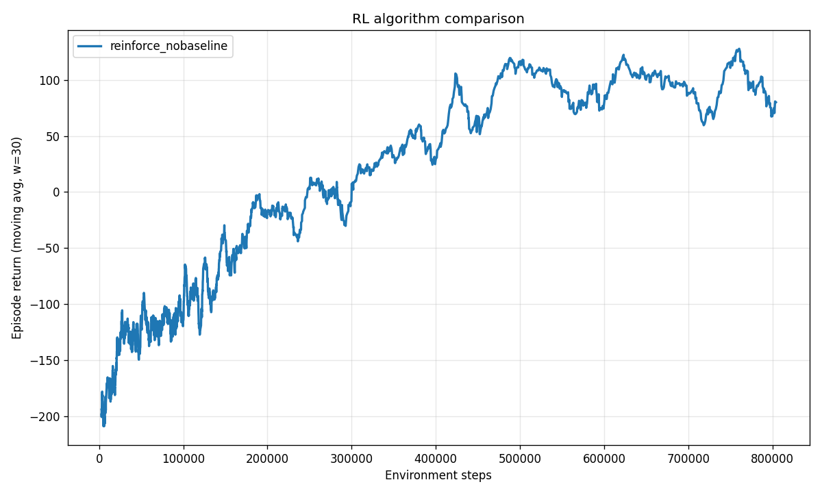
That's really all there is to coding REINFORCE. If we run the training script for 800k
steps, we see the reward increasing steadily before plateauing around 100:
Average episode reward over 800k training steps. The policy steadily improves before converging.
That's a good sign — our agent has learned a policy with high average reward. Let's deploy
it in practice. Instead of sampling from the learned distribution, we use a
greedy deterministic approach and pick the argmax of the categorical logits.
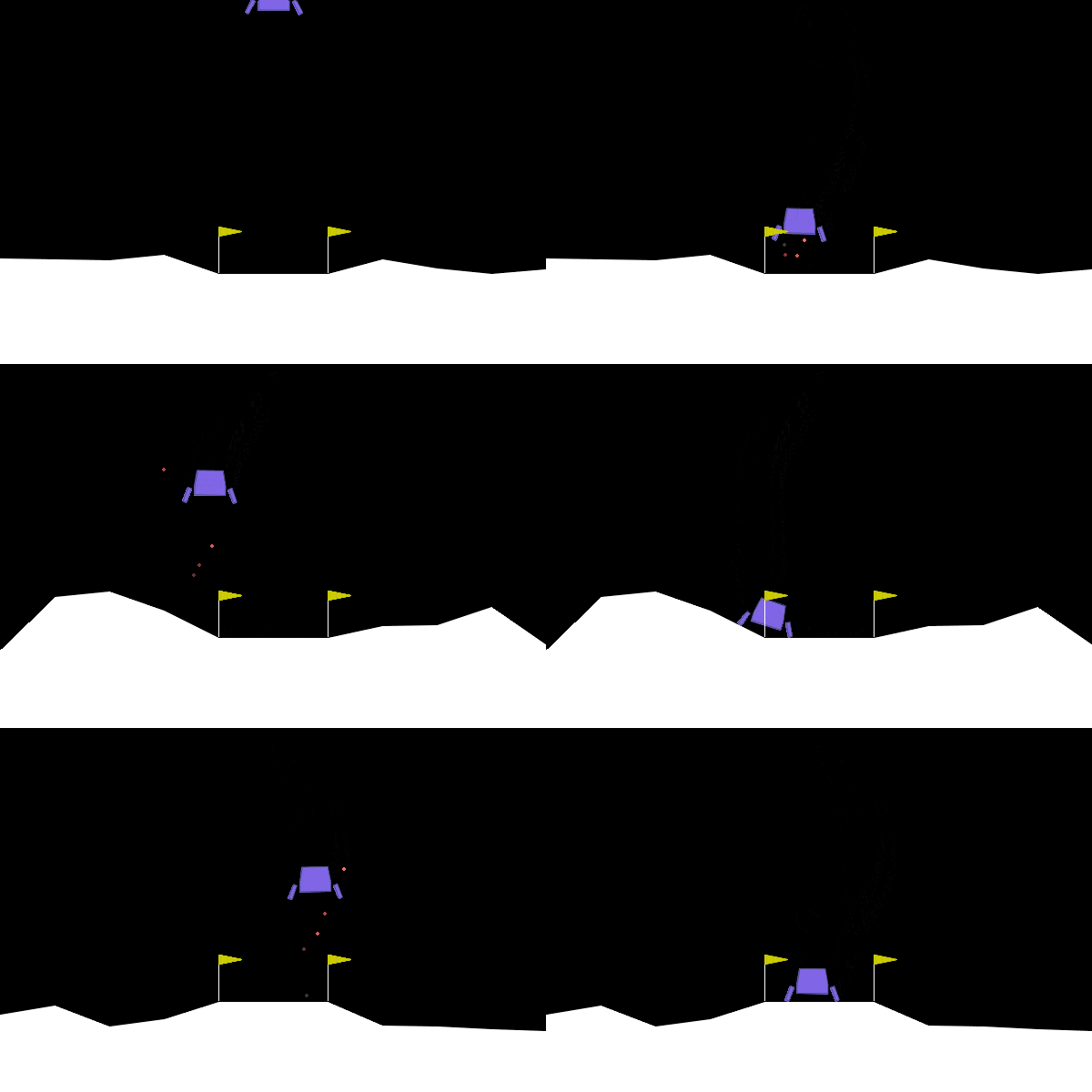
Gymnasium's RecordVideo wrapper (from gymnasium.wrappers) lets us
render and save episodes with a trained agent. The result is shown below:
Our REINFORCE agent successfully landing in various terrains and from various starting positions.
Conclusions and Next Steps
REINFORCE is a good foundation to have. It is a very common RL algorithm and usually a good
one to deploy if data scarcity or efficiency are not too big concerns. The Lunar Lander is
also a good first example for learning about Gymnasium and getting a feel for the code.
However, there are better algorithms out there. One vital issue with REINFORCE is its
high variance, which causes unstable training — in our policy gradient
expression we always weight by a full Monte Carlo return, which sums many random rewards.
Also, on-policy algorithms are very sample inefficient: we can fix this by
taking more gradient steps, but this leads to harder training and instability. Finally,
REINFORCE is relatively weak on long-horizon tasks.
We will continue this series next time with actor-critic methods.